4 Nutritional profiles
Code
library(ggplot2)
data <- get_model_data()
data$data_raw$timor_GN_raw$clusters <- paste0("FNP-", data$data_raw$timor_GN_raw$clusters)
data$data_raw$timor_AG_raw$clusters <- paste0("FNP-", data$data_raw$timor_AG_raw$clusters)


plot_profiles <- function(x) {
  means_dat <-
    x %>%
    dplyr::rename_with(~ stringr::str_to_title(.x), .cols = c(.data$zinc:.data$vitaminA)) %>%
    dplyr::rename(
      "Vitamin-A" = .data$Vitamina,
      "Omega-3" = .data$Omega3
    ) %>%
    tidyr::pivot_longer(c(Zinc:"Vitamin-A")) %>%
    dplyr::group_by(clusters, name) %>%
    dplyr::summarise(
      mean = mean(value, na.rm = TRUE),
      sd = sd(value, na.rm = TRUE),
      n = dplyr::n(),
      se = sd / sqrt(n),
      ci_lower = mean - qt(0.99, df = n - 1) * se,
      ci_upper = mean + qt(0.99, df = n - 1) * se
    )

  all_dat <-
    x %>%
    dplyr::rename_with(~ stringr::str_to_title(.x), .cols = c(.data$zinc:.data$vitaminA)) %>%
    dplyr::rename(
      "Vitamin-A" = .data$Vitamina,
      "Omega-3" = .data$Omega3
    ) %>%
    tidyr::pivot_longer(c(Zinc:"Vitamin-A"))


  ggplot() +
    ggpubr::theme_pubr()+
    geom_jitter(data = all_dat, mapping = aes(x = value, y = name, color = clusters), alpha = 0.01, size = 1, position = position_dodge(width = 0.5)) +
    geom_point(data = means_dat, mapping = aes(x = mean, y = name, color = clusters), size = 5, position = position_dodge(width = 0.5)) +
    labs(
      x = "",
      y = "",
      color = "Profiles"
    ) +
    ggplot2::theme(
      legend.position = "",
      plot.margin = unit(c(0, 0, 0, 0), "cm"),
      panel.grid = ggplot2::element_blank()
    ) +
    coord_cartesian(xlim = c(0, 5)) +
    scale_fill_manual(values = timor.nutrients::palettes$clusters_palette) +
    scale_color_manual(values = timor.nutrients::palettes$clusters_palette)
}

plots1 <- plot_profiles(data$data_raw$timor_AG_raw) #purrr::map(data$data_raw$timor_AG_raw, plot_profiles)

means_dat <-
  data$data_raw$timor_GN_raw %>%
  dplyr::rename_with(~ stringr::str_to_title(.x), .cols = c(.data$zinc:.data$vitaminA)) %>%
  dplyr::rename(
    "Vitamin-A" = .data$Vitamina,
    "Omega-3" = .data$Omega3
  ) %>%
  tidyr::pivot_longer(c(Zinc:"Vitamin-A")) %>%
  dplyr::group_by(clusters, name) %>%
  dplyr::summarise(
    mean = mean(value, na.rm = TRUE),
    sd = sd(value, na.rm = TRUE),
    n = dplyr::n(),
    se = sd / sqrt(n),
    ci_lower = mean - qt(0.99, df = n - 1) * se,
    ci_upper = mean + qt(0.99, df = n - 1) * se
  )

all_dat <-
  data$data_raw$timor_GN_raw %>%
  dplyr::rename_with(~ stringr::str_to_title(.x), .cols = c(.data$zinc:.data$vitaminA)) %>%
  dplyr::rename(
    "Vitamin-A" = .data$Vitamina,
    "Omega-3" = .data$Omega3
  ) %>%
  tidyr::pivot_longer(c(Zinc:"Vitamin-A"))

plots2 <-
  ggplot() +
  ggpubr::theme_pubr()+
  geom_jitter(data = all_dat, mapping = aes(x = value, y = name, color = clusters), alpha = 0.01, size = 1, position = position_dodge(width = 0.5)) +
  geom_point(data = means_dat, mapping = aes(x = mean, y = name, color = clusters), size = 5, position = position_dodge(width = 0.5)) +
  labs(
    x = "",
    y = "",
    color = "Profiles"
  ) +
  ggplot2::theme(
    legend.position = "",
    plot.margin = unit(c(0, 0, 0, 0), "cm"),
    panel.grid = ggplot2::element_blank()
  ) +
  coord_cartesian(xlim = c(0, 5)) +
  scale_fill_manual(values = timor.nutrients::palettes$clusters_palette) +
  scale_color_manual(values = timor.nutrients::palettes$clusters_palette) +
  annotate(
    'text',
    x = 3.5,
    y = 2.5,
    label = 'On average, FNP-3 provides enough\ncalcium for 2.2 people per 1kg of catch,\nwhile FNP-1 and FNP-2 support\n0.4 and 0.6 people, respectively',
    size = 2.75
  ) +
  #annotate(
  #  'rect',
  #  xmin = 0,
  #  ymin = 0.5,
  #  ymax = 1.5,
  #  xmax = 4.5,
    #alpha = 0.5,
  #  color = rgb(0, 0, 0, alpha = 0.85),
   # linewidth = 0.3,
    #fill = "transparent",
    #linetype = 2
  #) +
  annotate(
    'curve',
    x = 3.4, # Play around with the coordinates until you're satisfied
    y = 1.8,
    yend = 1.3,
    xend = 2.45,
    col = 'black',
    curvature = -0.05,
    linewidth = 0.3,
    arrow = arrow(length = unit(0.25, 'cm'))
  )


plots <-
  list(
    plots2 + ggplot2::labs(subtitle = "Gill nets"),
    plots1 + ggplot2::labs(subtitle = "Other gears")
  )

legend_plot <- cowplot::get_legend(plots[[1]] +
                                     ggplot2::theme(
                                       legend.position = "right",
                                       legend.key.size = ggplot2::unit(0.55, "cm"),
                                       legend.title = ggplot2::element_text(size = 12)
                                     ))
combined_plots <- cowplot::plot_grid(plotlist = plots, ncol = 2, labels = "AUTO")

x_label <- cowplot::draw_label("NDS per 1kg of catch", x = 0.5, y = 0.05)
y_label <- cowplot::draw_label("Nutrient", x = 0.04, y = 0.5, angle = 90)

final_plot <-
  cowplot::plot_grid(
    combined_plots,
    legend_plot,
    ncol = 2,
    rel_widths = c(1, 0.15),
    scale = 0.9
  ) +
  x_label +
  y_label

final_plot
Code
kmean_plots <- data$kmeans_plots

plots <-
  list(
    kmean_plots$kmeans_timor_GN + ggplot2::labs(subtitle = "Gill nets"),
    kmean_plots$kmeans_timor_AG + ggplot2::labs(subtitle = "Other gears")
  )

plots <- lapply(plots, function(x) {
  x +
    ggpubr::theme_pubr()+
    ggplot2::theme(
      legend.position = "none",
      plot.margin = unit(c(0, 0, 0, 0), "cm"),
      panel.grid = ggplot2::element_blank()
    ) +
    ggplot2::labs(
      fill = "Profiles",
      color = "Profiles"
    )+
    ggplot2::scale_color_manual(
      values = timor.nutrients::palettes$clusters_palette,
      labels = function(x) paste0("FNP-", x)
    ) +
    ggplot2::scale_fill_manual(
      values = timor.nutrients::palettes$clusters_palette,
      labels = function(x) paste0("FNP-", x)
    )
  })

legend_plot <- cowplot::get_legend(plots[[1]] +
  ggplot2::theme(
    legend.position = "right",
    legend.key.size = ggplot2::unit(0.6, "cm"),
    legend.title = ggplot2::element_text(size = 12)
  ))
combined_plots <- cowplot::plot_grid(plotlist = plots, ncol = 2, labels = "AUTO")

# x_label <- cowplot::draw_label("False positive rate\n(1 - Specificity)", x = 0.5, y = 0.05)
# y_label <- cowplot::draw_label("True positive rate\n(Sensitivity)", x = 0.02, y = 0.5, angle = 90)

final_plot <-
  cowplot::plot_grid(
    combined_plots,
    legend_plot,
    ncol = 2,
    rel_widths = c(1, 0.1),
    scale = 0.9
  )

final_plot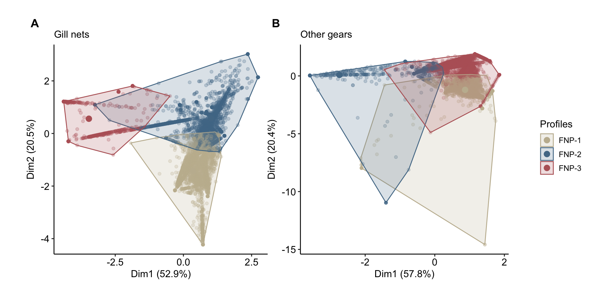
Code
timor.nutrients::perm_results %>%
  dplyr::bind_rows(.id = "subset") %>%
  dplyr::mutate(dplyr::across(c(SumOfSqs, R2, statistic), ~ round(.x, 2)),
    p.value = ifelse(p.value <= 0.001, "< 0.001", p.value),
    subset = stringr::str_remove(subset, "_perm"),
    subset = stringr::str_replace(subset, "timor", "mainland")
  ) %>%
  reactable::reactable(
    theme = reactablefmtr::fivethirtyeight(centered = TRUE),
    groupBy = "subset",
    defaultExpanded = TRUE,
    pagination = FALSE,
    compact = FALSE,
    borderless = FALSE,
    striped = FALSE,
    defaultColDef = reactable::colDef(
      align = "center"
    ),
    columns = list(
      subset = reactable::colDef(
        minWidth = 120
      )
    )
  )
Code
models_auc <-
  timor.nutrients::model_outputs %>%
  purrr::map(purrr::pluck(8)) %>%
  dplyr::bind_rows(.id = "subset") %>%
  dplyr::select(-estimator) %>%
  tidyr::pivot_wider(names_from = subset, values_from = estimate)


plots <-
  list(
    timor.nutrients::model_outputs$model_timor_GN$roc_curves + ggplot2::labs(subtitle = paste0("Gill nets", " (", models_auc$model_timor_GN, ")")),
    timor.nutrients::model_outputs$model_timor_AG$roc_curves + ggplot2::labs(subtitle = paste0("Other gears", " (", models_auc$model_timor_AG, ")"))
  )
plots <- lapply(plots, function(x) {
  x +
   ggpubr::theme_pubr()+
    ggplot2::theme(
      panel.grid = ggplot2::element_blank(),
      legend.position = "none",
      plot.margin = unit(c(0, 0, 0, -0.1), "cm")
    ) +
    ggplot2::coord_cartesian(expand = T) +
    ggplot2::labs(x = "", y = "", color = "Profiles")+
      ggplot2::scale_color_manual(
      values = timor.nutrients::palettes$clusters_palette,,
      labels = function(x) paste0("FNP-", x)
    ) +
    ggplot2::scale_fill_manual(
      values = timor.nutrients::palettes$clusters_palette,,
      labels = function(x) paste0("FNP-", x)
    )
})
legend_plot <- cowplot::get_legend(plots[[1]] +
  ggplot2::theme(
    legend.position = "right",
    legend.key.size = ggplot2::unit(0.8, "cm"),
    legend.title = ggplot2::element_text(size = 12)
  ))
combined_plots <- cowplot::plot_grid(plotlist = plots, ncol = 2, labels = "AUTO", vjust = 0.2)

x_label <- cowplot::draw_label("False positive rate (1 - Specificity)", x = 0.5, y = 0.05)
y_label <- cowplot::draw_label("True positive rate (Sensitivity)", x = 0.02, y = 0.5, angle = 90)

final_plot <-
  cowplot::plot_grid(
    combined_plots,
    legend_plot,
    ncol = 2,
    rel_widths = c(1, 0.15),
    scale = 0.9
  ) +
  x_label +
  y_label

final_plot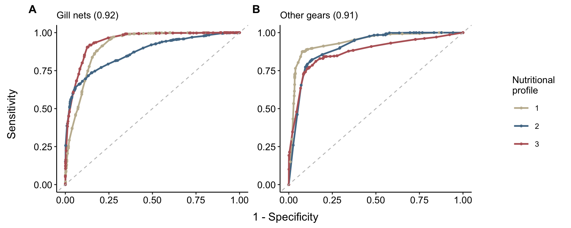
Code
models_metrics <-
  timor.nutrients::model_outputs %>%
  purrr::map(purrr::pluck(4)) %>%
  purrr::imap(~ summary(.x)) %>%
  dplyr::bind_rows(.id = "subset") %>%
  dplyr::select(-.estimator) %>%
  tidyr::pivot_wider(names_from = subset, values_from = .estimate) %>%
  dplyr::rename(metric = .metric) %>%
  na.omit()


dplyr::bind_rows(models_auc, models_metrics) %>%
  dplyr::rename(
    "Other gears" = model_timor_AG,
    "Gill nets" = model_timor_GN
  ) %>%
  dplyr::mutate(dplyr::across(.cols = dplyr::where(is.numeric), ~ round(.x, 2))) %>%
  reactable::reactable(
    theme = reactablefmtr::fivethirtyeight(centered = TRUE),
    defaultExpanded = TRUE,
    pagination = FALSE,
    compact = FALSE,
    borderless = FALSE,
    striped = FALSE,
    defaultColDef = reactable::colDef(
      align = "center"
    ),
    columns = list(
      metric = reactable::colDef(
        minWidth = 120
      )
    )
  )
Code
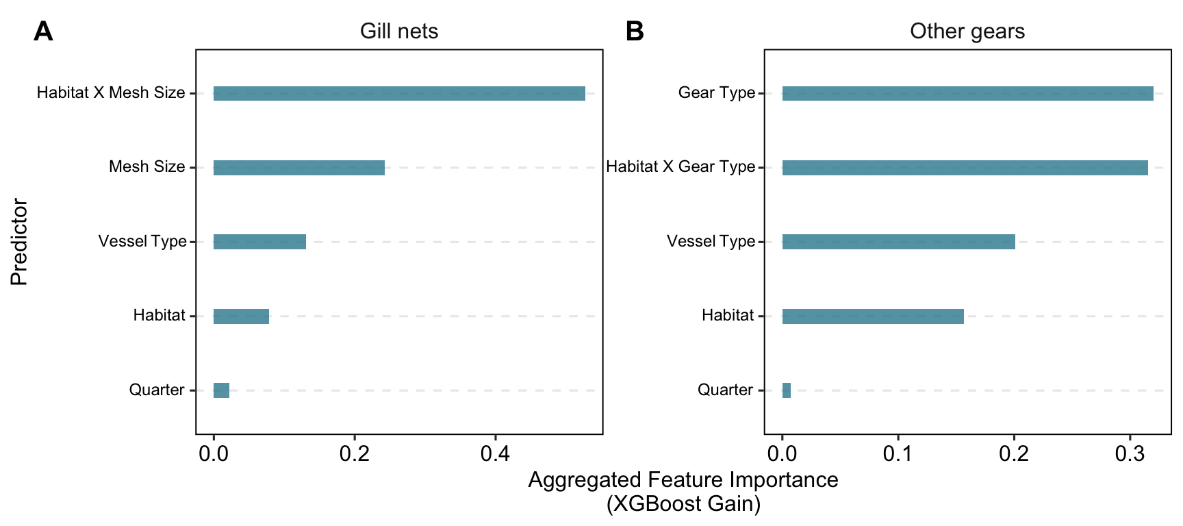
importance_ag <-
  model_outputs$model_timor_AG$fit %>%
  workflows::extract_fit_parsnip() %>%
  vip::vi() %>%
  dplyr::mutate(
    category = dplyr::case_when(
      stringr::str_detect(Variable, "gear_type") ~ "gear_type",
      stringr::str_detect(Variable, "habitat_gear") ~ "habitat_gear",
      stringr::str_detect(Variable, "habitat") ~ "habitat",
      stringr::str_detect(Variable, "quarter") ~ "quarter",
      stringr::str_detect(Variable, "vessel_type") ~ "vessel_type",
      TRUE ~ "other"
    )
  ) %>%
  dplyr::group_by(category) %>%
  dplyr::summarize(Aggregated_Importance = sum(Importance)) %>%
  dplyr::arrange(dplyr::desc(Aggregated_Importance))

importance_gn <-
  model_outputs$model_timor_GN$fit %>%
  workflows::extract_fit_parsnip() %>%
  vip::vi() %>%
  dplyr::mutate(
    category = dplyr::case_when(
      stringr::str_detect(Variable, "mesh_size") ~ "mesh_size",
      stringr::str_detect(Variable, "habitat_mesh") ~ "habitat_mesh",
      stringr::str_detect(Variable, "habitat") ~ "habitat",
      stringr::str_detect(Variable, "quarter") ~ "quarter",
      stringr::str_detect(Variable, "vessel_type") ~ "vessel_type",
      TRUE ~ "other"
    )
  ) %>%
  dplyr::group_by(category) %>%
  dplyr::summarize(Aggregated_Importance = sum(Importance)) %>%
  dplyr::arrange(dplyr::desc(Aggregated_Importance))

importance_plot <-
  dplyr::bind_rows(
    importance_ag %>% dplyr::mutate(model = "Other gears"),
    importance_gn %>% dplyr::mutate(model = "Gill nets")
  ) %>%
  dplyr::mutate(category = dplyr::case_when(category == "habitat_gear" ~ "habitat x gear type",
                                            category == "habitat_mesh" ~ "habitat x mesh size",
                                            TRUE ~ category),
                category = stringr::str_replace(category, "_", " "),
                category = stringr::str_to_title(category)
                ) %>%
  ggplot(aes(x = reorder(category, Aggregated_Importance), y = Aggregated_Importance)) +
  ggpubr::theme_pubr(border = TRUE) +
  facet_wrap(~model, scales = "free") +
  geom_col(width = 0.2, fill = "#1c8097", alpha = 0.75) +
  coord_flip() +
  labs(
    x = "Predictor",
    y = "Aggregated Feature Importance\n(XGBoost Gain)"
  ) +
  theme(
    panel.grid.major.y = element_line(linetype = "dashed"),
    strip.background = ggplot2::element_blank(),
    strip.text = element_text(size = 12),
    axis.text.y = ggtext::element_markdown(size = 9),
    panel.spacing = unit(0.1, "lines"),
  )

cowplot::ggdraw(importance_plot) +
  cowplot::draw_plot_label(
    label = c("A", "B"),
    x = c(0.02, 0.52),  # Adjust the x position of labels
    y = c(0.98, 0.98),  # Adjust the y position of labels
    size = 15
  )
Code
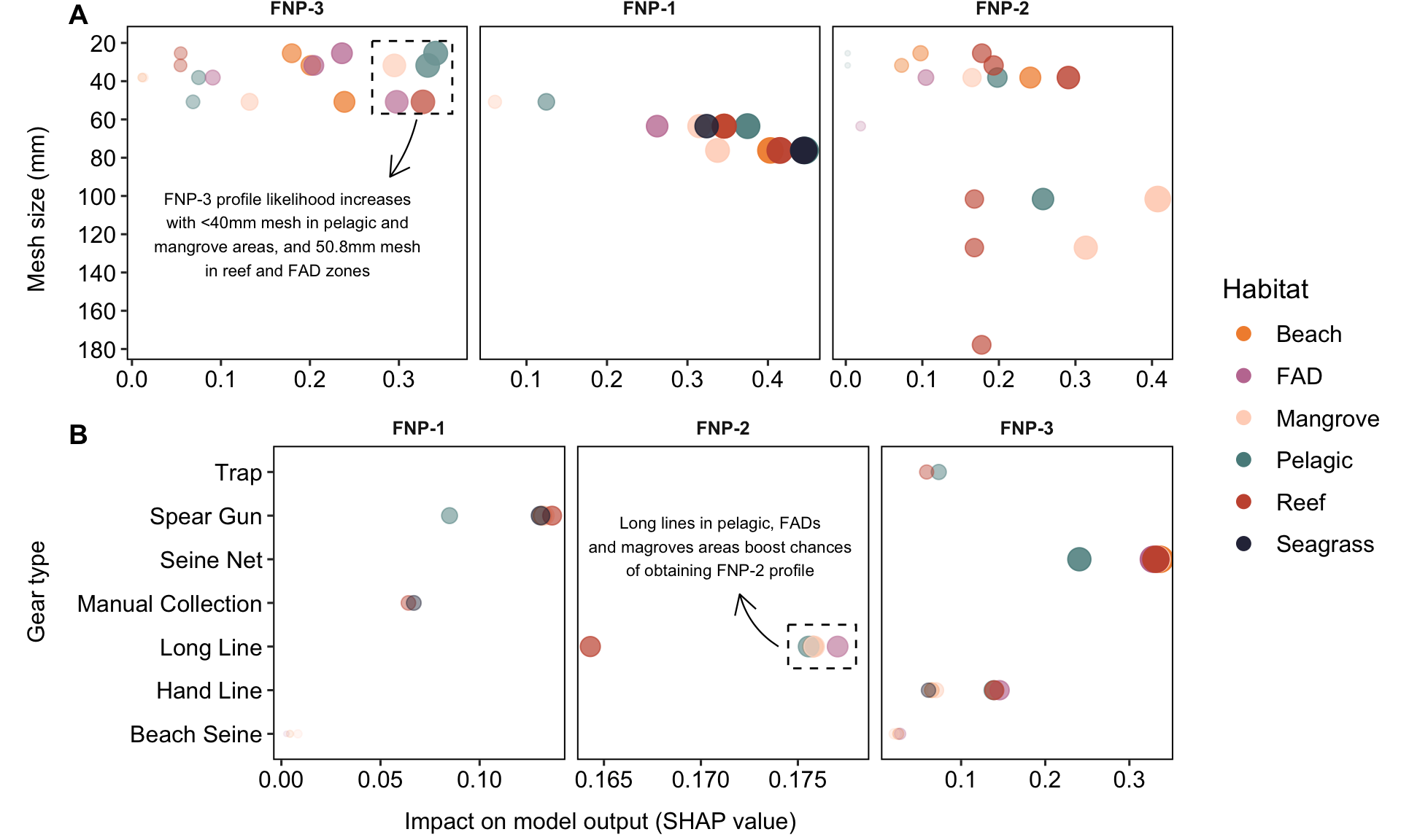
sha_Mgn <- shapviz::shapviz(timor.nutrients::shap_results$model_timor_GN)

annotation_data <- data.frame(
  profile = "FNP-3",
  x = 0.175,
  y = 120,
  label = 'FNP-3 profile likelihood increases\nwith <40mm mesh in pelagic and\nmangrove areas, and 50.8mm mesh\nin reef and FAD zones'
)

p2 <-
  sha_Mgn %>%
  purrr::map(get_shaps, model_type = "gn") %>%
  dplyr::bind_rows(.id = "profile") %>%
  dplyr::mutate(profile = stringr::str_replace(profile, ".pred_", "FNP-")) %>%
  dplyr::group_by(profile, habitat_fact, mesh_fact) %>%
  dplyr::summarise(mesh_shap = median(mesh_shap, na.rm = TRUE)) %>%
  dplyr::ungroup() %>%
  dplyr::filter(mesh_shap > 0) %>%
  dplyr::mutate(habitat_fact = dplyr::case_when(habitat_fact == "Deep" ~ "Pelagic", TRUE ~ habitat_fact)) %>%
  ggplot2::ggplot(ggplot2::aes(mesh_shap, mesh_fact, color = habitat_fact)) +
  facet_grid(. ~ factor(profile, levels = c("FNP-1", "FNP-2", "FNP-3")), scales = "free") +
  ggplot2::geom_point(ggplot2::aes(alpha = sqrt(mesh_shap), size = mesh_shap)) +
  ggpubr::theme_pubr(border = TRUE) +
  ggplot2::scale_color_manual(values = c("#f28f3b", "#c27ba0", "#ffd5c2", "#588b8b", "#c8553d", "#2d3047", "#007ea7")) +
  ggplot2::coord_cartesian(expand = TRUE) +
  ggplot2::scale_y_reverse(n.breaks = 10) +
  ggplot2::labs(color = "Habitat") +
  ggplot2::theme(
    panel.grid = ggplot2::element_blank(),
    strip.background = ggplot2::element_blank(),
    strip.text.x = ggplot2::element_text(face = "bold")
  ) +
  ggplot2::guides(
    color = ggplot2::guide_legend(override.aes = list(size = 3)),
    alpha = "none",
    size = "none"
  ) +
  ggplot2::geom_text(
    data = annotation_data,
    aes(x = x, y = y, label = label),
    size = 3,
    fontface = "plain",
    inherit.aes = FALSE
  ) +
  ggplot2::geom_rect(
    data = annotation_data,
    aes(xmin = 0.27, xmax = 0.36, ymin = 19, ymax = 57),
    fill = "white",
    alpha = 0.2,
    color = "black",
    inherit.aes = FALSE,
    linetype = "dashed"
  ) +
  ggplot2::geom_curve(
    data = annotation_data,
    aes(x = 0.32, y = 60, xend = 0.29, yend = 90),
    curvature = -0.1,
    color = 'black',
    linewidth = 0.4,
    arrow = arrow(length = unit(0.4, 'cm')),
    inherit.aes = FALSE
  ) +
  ggplot2::labs(x = "", y = "")


leg <- cowplot::get_legend(p2 +
                             ggplot2::theme(
                               plot.margin = unit(c(2, 0, 0, 0.9), "cm"),
                               # legend.title = ggplot2::element_text(size = 11),
                               legend.position = "right",
                               legend.direction = "vertical",
                               legend.justification = "right",
                               legend.box.just = "right",
                               legend.background = element_rect(fill = "transparent", colour = NA),
                               legend.box.background = element_rect(fill = "transparent", colour = NA)
                             ))

base_plot <-
  cowplot::plot_grid(
    p2 + theme(
      legend.position = "none",
      plot.margin = unit(c(-0.2, 0.5, 0, 0.9), "cm")
    ),
    ncol = 1,
    labels = c("A", "B"),
    hjust = -3.5,
    vjust = 1.2,
    align = "v"
  )

grid <-
  cowplot::plot_grid(
    base_plot,
    nrow = 1
  )

pp1 <-
  cowplot::ggdraw() +
  cowplot::draw_plot(grid) +
  cowplot::draw_label("Mesh size (mm)", x = 0.03, y = 0.7, angle = 90, hjust = 1, size = 12)

sha_Mag <- shapviz::shapviz(timor.nutrients::shap_results$model_timor_AG)

process_shap <-
  sha_Mag %>%
  purrr::map(get_shaps, model_type = "ag") %>%
  dplyr::bind_rows(.id = "profile") %>%
  tidyr::separate(habitat_gear_fact, into = c("habitat", "gear_fact"), sep = "_") %>%
  dplyr::mutate(
    gear_fact = stringr::str_to_title(gear_fact),
    profile = stringr::str_replace(profile, ".pred_", "FNP-"),
    habitat_gear_fact = paste0(habitat, " x ", gear_fact),
    habitat_gear_fact = stringr::str_replace(habitat_gear_fact, "Deep", "Pelagic")
  )

to_group <-
  process_shap %>%
  dplyr::mutate(
    zero_dist = 0 - abs(gear_fact_shap)
  ) %>%
  dplyr::group_by(gear_fact) %>%
  dplyr::summarise(zero_dist = mean(zero_dist)) %>%
  dplyr::slice_max(order_by = zero_dist, n = 15) %>%
  magrittr::extract2("gear_fact")

annotation_data <- data.frame(
  profile = "FNP-2",
  x = 0.171,
  y = 5.3,
  label = 'Long lines in pelagic, FADs\nand magroves areas boost chances\nof obtaining FNP-2 profile'
)

p2 <-
  process_shap %>%
  dplyr::mutate(gear_fact_shap = ifelse(gear_fact_shap %in% to_group, "Others", gear_fact_shap)) %>%
  dplyr::group_by(profile, gear_fact, habitat_fact) %>%
  dplyr::summarise(gear_fact_shap = median(gear_fact_shap, na.rm = TRUE)) %>%
  dplyr::ungroup() %>%
  dplyr::filter(gear_fact_shap > 0) %>%
  dplyr::mutate(habitat_fact = dplyr::case_when(habitat_fact == "Deep" ~ "Pelagic", TRUE ~ habitat_fact)) %>%
  ggplot2::ggplot(ggplot2::aes(gear_fact_shap, gear_fact, color = habitat_fact)) +
  facet_grid(. ~ profile, scales = "free") +
  ggplot2::geom_point(ggplot2::aes(alpha = sqrt(gear_fact_shap), size = gear_fact_shap)) +
  ggpubr::theme_pubr(border = TRUE) +
  ggplot2::scale_color_manual(values = c("#f28f3b", "#c27ba0", "#ffd5c2", "#588b8b", "#c8553d", "#2d3047", "#007ea7")) +
  ggplot2::coord_cartesian(expand = TRUE) +
  ggplot2::scale_x_continuous(n.breaks = 4) +
  ggplot2::labs(color = "Habitat") +
  ggplot2::theme(
    panel.grid = ggplot2::element_blank(),
    strip.background = ggplot2::element_blank(),
    strip.text.x = ggplot2::element_text(face = "bold")
  ) +
  ggplot2::geom_text(
    data = annotation_data,
    aes(x = x, y = y, label = label),
    size = 3,
    fontface = "plain",
    inherit.aes = FALSE
  ) +
  ggplot2::geom_curve(
    data = annotation_data,
    aes(x = 0.174, y = 3, xend = 0.172, yend = 4.2),
    curvature = -0.2,
    color = 'black',
    linewidth = 0.4,
    arrow = arrow(length = unit(0.4, 'cm')),
    inherit.aes = FALSE
  ) +
  ggplot2::geom_rect(
    data = annotation_data,
    aes(xmin = 0.1745, xmax = 0.178, ymin = 2.5, ymax = 3.5),
    fill = "white",
    alpha = 0.2,
    color = "black",
    inherit.aes = FALSE,
    linetype = "dashed"
  ) +
  ggplot2::guides(
    color = ggplot2::guide_legend(override.aes = list(size = 3)),
    alpha = "none",
    size = "none"
  ) +
  ggplot2::labs(x = "", y = "")

leg <- cowplot::get_legend(p2 +
                             ggplot2::theme(
                               plot.margin = unit(c(2, 0, 0, 0.9), "cm"),
                               # legend.title = ggplot2::element_text(size = 11),
                               legend.position = "right",
                               legend.direction = "vertical",
                               legend.justification = "right",
                               legend.box.just = "right",
                               legend.background = element_rect(fill = "transparent", colour = NA),
                               legend.box.background = element_rect(fill = "transparent", colour = NA)
                             ))

base_plot <-
  cowplot::plot_grid(
    p2 + theme(
      legend.position = "none",
      plot.margin = unit(c(-0.2, 0.5, 0, 0.9), "cm")
    ),
    ncol = 1,
    labels = c("B", "D"),
    hjust = -3.5,
    vjust = 1.2,
    align = "v"
  )

grid <-
  cowplot::plot_grid(
    base_plot,
    nrow = 1
  )

pp2 <-
  cowplot::ggdraw(ylim = c(-.05, NA)) +
  cowplot::draw_plot(grid) +
  cowplot::draw_label("Gear type", x = 0.03, y = 0.7, angle = 90, hjust = 1, size = 12) +
  cowplot::draw_label("Impact on model output (SHAP value)", x = 0.5, y = 0, size = 12)

# Extract the shared legend with larger text and key sizes
shared_legend <- cowplot::get_legend(
  p2 +
    ggplot2::theme(
      legend.position = "right",                # Position the legend on the right
      legend.direction = "vertical",           # Vertical orientation
      legend.justification = "center",
      legend.box.just = "center",
      legend.text = ggplot2::element_text(size = 12),  # Increase text size
      legend.title = ggplot2::element_text(size = 14), # Increase title size
      legend.key.size = unit(1.5, "lines"),    # Increase legend key size
      legend.background = ggplot2::element_rect(fill = "transparent", colour = NA),
      legend.box.background = ggplot2::element_rect(fill = "transparent", colour = NA)
    )
)

# Remove legends from individual plots
pp1_no_legend <-
  pp1 +
  ggplot2::theme(legend.position = "none")

pp2_no_legend <-
  pp2 +
  ggplot2::theme(legend.position = "none")

# Combine the two plots vertically without legends
plots_combined <- cowplot::plot_grid(
  pp1_no_legend,
  pp2_no_legend,
  align = "v",          # Align the plots vertically
  ncol = 1,             # Stack in one column
  rel_heights = c(1, 1) # Adjust heights if necessary
)

# Add the shared legend to the right
final_plot <- cowplot::plot_grid(
  plots_combined,
  shared_legend,
  ncol = 2,             # Add legend to the right of the plots
  rel_widths = c(3, 0.5) # Adjust widths for the plots and legend
)

# Display the final plot
print(final_plot)